Now that we’ve covered the design/layout, procedure, and instrument calibration and traceability for our experiment, it’s time to start analyzing our data.
Section 4.3: Data Analysis and Uncertainties
The goals for this section of your report are
- Show us what happens to a raw data point prior to being reported, such that the raw data can be analyzed by someone, somewhere else.
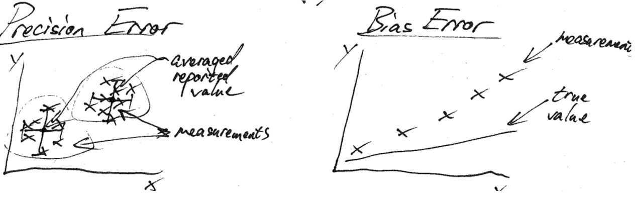
- Show us where uncertainties of the reported values come from (i.e. bias error, precision error, etc.)
- Quantify how confident you are in the reported measurements.
- Conform to ASTM Standard E2586 – Standard Practice for Calculating and Using Basic Statistics. You can download the pdf for free while on campus.
How do we quantify confidence? This is where we realize the value of our engineering education. We’ve all calculated a standard deviation by now and know that 68% of the measurements fall within ±σ of the mean (a.k.a. a coverage factor of 1), 95% lie within ±2σ (a.k.a. a coverage factor of 2), and 99.7% lie within ±3σ (a.k.a. a coverage factor of 3). While it’s straightforward to calculate the coverage factor for every steady state measurement you take. You should also do a repeatability test at several points to double-check. A classic example is that someone states that the uncertainty has a coverage factor of 2 (99.7% of all measurements fall with y of mean); however, this is only a repeatability test of the precision error. You still need to propagate instrument uncertainties to determine the bias error.
This portion of the lesson contains a considerable amount of math as we go through the Root-Sum-Square (RSS) method and what it means for uncertainty propagation. Remember that we can do this math by hand or with a computer program, which will estimate the uncertainties numerically. Here’s a link to the hand-written notes: lesson-6-lecture-notes.
Here’s an interesting problem — what if your measurement changes bases on the direction that you took it? Some measurements will, this is a type of Bias error that is specific to systems (systematic error) known as hysteresis. It’s common for thermal systems with components that slowly heat up over time. How can you account for (or at least rule out) this type of error as an experimentalist? One approach is to randomize your measurement points. Don’t proceed logically from point to point while steadily increasing a value — this will cause hysteresis to appear as a bias error that is much more difficult to systematically remove. Randomizing your measurement points causes hysteresis to appear as precision error — much easier to account for.
By the end of lab today you should have the following completed:
- Have repeated a measurement on the way to 5 trials at the same operating point (you should have at least one repeatability test for each operating regime of the experiment).
- Tested for hysteresis by measuring the same point from different directions and/or randomizing the measurement points.
- Use the Root-Sum-Squares (RSS) method to estimate the total uncertainty (precision and bias) for one of your data points (everyone is required to show this in their reports).
- Drafted section 4.3 of your report on Data Analysis and Uncertainty Propagation.
Next time we’ll focus on visualizing your measurements.