Welcome to the ME 527 Macroscale Thermodynamics Page
ME 527 Macroscale Thermodynamics is a classic course at WSU that compliments ME 526 Microscale Thermodynamics (a.k.a. Statistical Thermodynamics). Macroscale thermo covers three key topics:
- A rigorous review of Thermodynamic Law from the introductory thermodynamics courses. Emphasis is on process — from system definition, assumption application, and derivation of balances. After this, a graduate student should feel comfortable teaching the beginner course with a mastery of the thermodynamic problem solving process. We cover what is easily solvable by hand, and quickly understand how and why software is so important in thermodynamics.
- The structure of thermophysical properties — understanding where thermophysical properties come from, definitions, inter-relationships, and equations of state for pure fluids and mixtures.
- Entropy/Energy optimization — we will understand the develop the bridge between equilibrium and non-equilibrium (thermodynamic versus transport) properties and build a foundation in non-equilibrium thermodynamics necessary to apply Bejan’s constructal theories in his Advanced Engineering Thermodynamics textbook. We will then optimize the structure of systems from fundamental law. Snowflakes, trees, energy grids — nothing that follows the laws of thermodynamics is off limits.
Here is the course syllabus for Spring 2018: ME 527 syllabus Sp2018 In the sections below you’ll find summaries and key takeaways from the course.
Reviewing the Laws of Thermodynamics
It may indeed be law that all legalistic processes optimize into a tree-like hierarchy. This, in a sense, is the essence of Bejan’s “Constructal Law” that all systems, when left free to optimize, will become tree-like. Over the years the laws of thermodynamics have done something similar. Here is my thermodynamic process decision tree that can solve basically any thermodynamic problem:
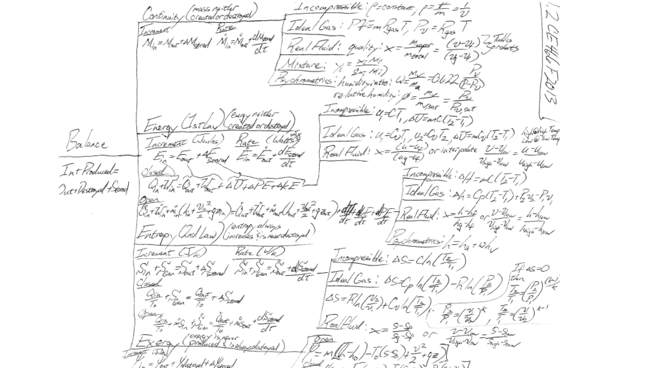
I know, it’s overwhelming if you’re not comfortable with thermo. Rather than thinking about this as a decision tree, let’s break it down into a process defined by the following layers:
- System definition: You basically have four options — open or closed to mass flow, and with either an open or closed system you can do an incremental or rate balance. Draw a line showing this system and the relevant flows that cross the system boundary.
- List your assumptions: When you get good at this, your assumptions will list out in a natural order that allows you to simplify your balance. I usually list which system I’ve selected as the first assumption, what kindof heat transfer problem it is (adiabatic, given, the thing being solved for, or a rate problem), what kind of work problem it is (PV, shaft, electrical, etc), whether kinetic or potential energy terms are significant, and finally the fluid model I’ll be assuming.
- Derive your balance: Write out that entire equation at the base of the tree above — IN+PRODUCED=OUT+DESTROYED+STORED — you can balance any quantifiable thing in the universe with that equation. Applied to energy and mass it’s just IN=OUT+STORED. And it could be rate based (/time) or over an increment in time. Write out all of the possible terms, then apply your assumptions to simplify to only the relevant terms being considered for your problem.
- Apply your fluid model: With your balances fully simplified, you now have to input thermodynamic properties in order to solve the balance. This is application of the fluid model. I teach three basic models: Real, ideal, incompressible. Those three will cover just about anything. When in doubt, just use a real model and software — it’s the best you can do! Ideal and incompressible are only still useful for computational efficiency.
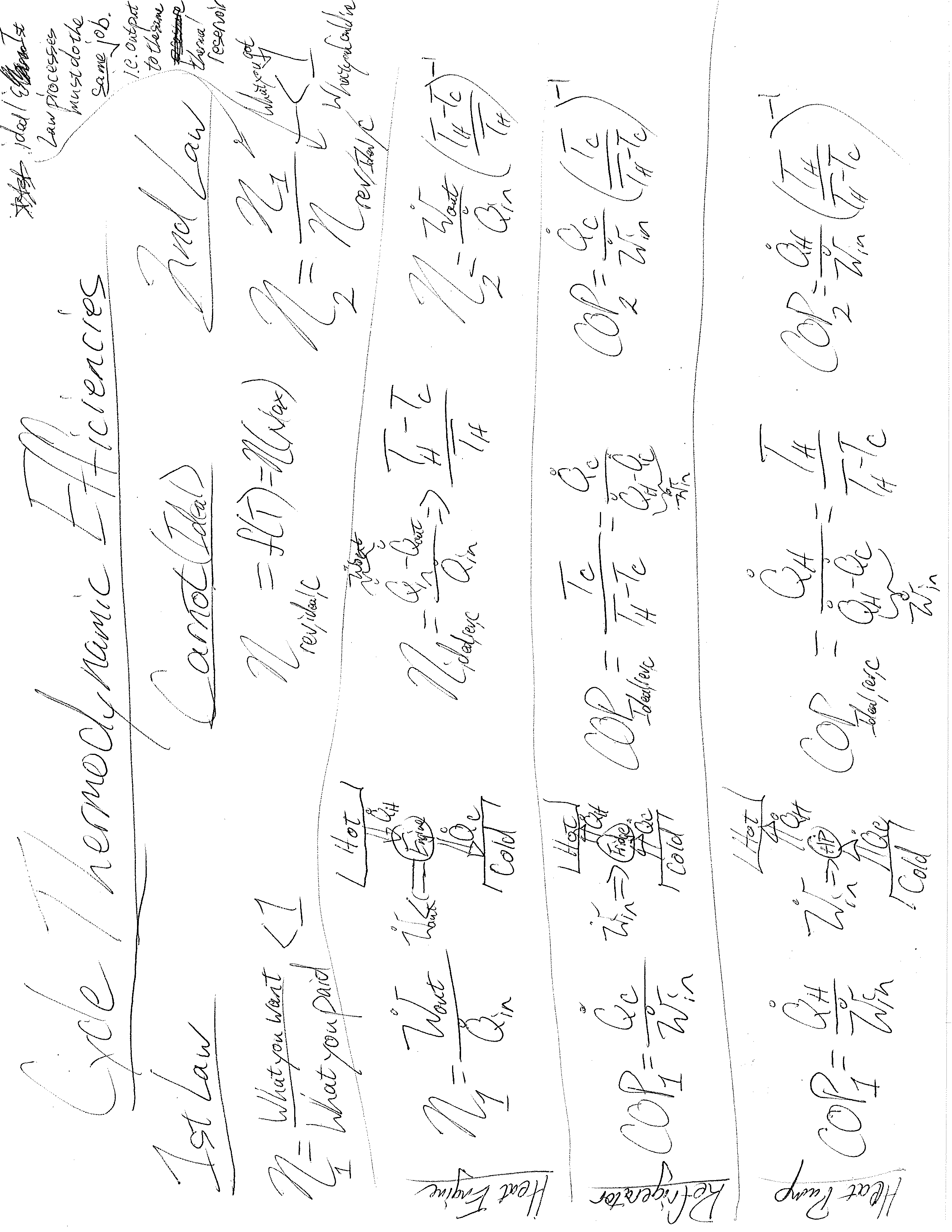
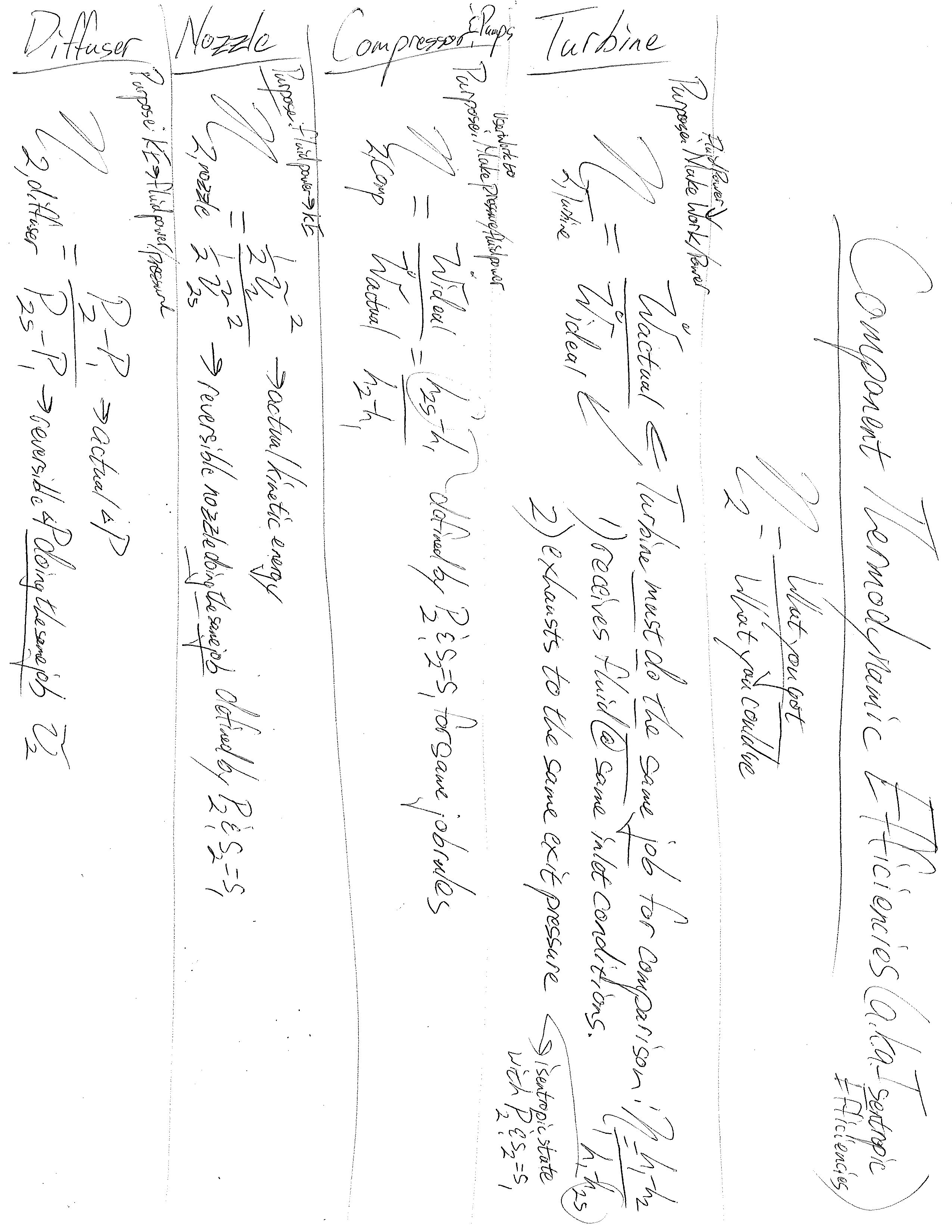
Understanding this process is the primary emphasis when reviewing the first law of thermodynamics and energy balances. The second law brings up additional considerations not included in our tree-like hierarchy of balances: the maximum efficiencies of components and cycles. I have not found a nice process or spectrum showing the different kinds of efficiencies and how derived. This is a problem as it is often difficult to determine which of competing systems perform better as it is somewhat an apples to apples question. Here’s a start to a thermodynamic efficiency diagram:
The problem solving process for balancing entropy is the same as that described for energy above. We just have to remember how entropy flows across system boundaries (with heat or mass) and is stored within systems. Much like energy, entropy has multiple forms (see Renyi, information, and Tsallis entropies) that can be stored and balanced in a system.
2nd Law concepts seem to be more difficult for mechanical engineering students than 1st Law. Part of this is the order in which the concepts are taught. For most of us though mechanistic systems utilizing pressure and a change in volume to accomplish work are more intuitive than thermal systems that utilize temperature and a change in entropy to accomplish heat flow. Section 2.6 in Bejan’s textbook, “A Heat Transfer Man’s 2 Axioms” does a wonderful job of helping us to see this duality of the 1st and 2nd laws.
The goal for the student is that before leaving the 2nd law, they are able to realize this beautiful duality by showing that the maximum entropy generation possible for a system is equal to the maximum possible work production — this is the core essence of availability/exergy analysis and a key point we continue to return to as we analyze cycles.
A key aspect to understanding thermodynamic cycles is to first understand the temperature gradient (analogous to an elevation gradient for an Olympic winter event) that the cycle is operating within. This temperature gradient, when presented on a T-s diagram shows that perfect cycles are indeed a square, and that power producing cycles proceed around the square in clock-wise fashion and power consuming (refrigeration) cycles move in counter-clockwise rotation. All inefficiencies we bring into cycles in our efforts to design an actual system cause deviations from this square.
To conclude our review of the thermodynamic laws and balances we directly address exergy by completing the balance (the final branch of our thermodynamic tree above). We realize that exergy is not new, and in many ways is simply a more efficient balance that combines the 1st and 2nd laws.
Table of Contents
The Structure of Thermophysical Properties, Equations of State, and Mixtures
When we reviewed the laws of thermodynamics we used just three fluid models: real fluid properties from software or tables, the ideal gas fluid model, and the incompressible substance fluid model. We really didn’t discuss where they came from, just simply where they were applied and the rules for each. Yet, all of the balances of the thermodynamic laws rely on our abilities to implement property models consistent with the thermodynamic laws for our inputs to these balances.
I’ve seen thermophysical properties taught from many different angles. My approach is primarily historical, so as to empathize with mind-set of the researchers who came up with the original models. Here’s a writeup on The Ideal Early Days of Thermophysical Properties. Which leads to The not so ideal Later Days of Thermophysical Properties. Along the way we build from the most basic ideal-gas equation of state (EOS), to the generalized van Der Waals and cubic class of EOS. We show the origins of the virial EOS in statistical mechanics. We culminate in modern multi-parameter EOS.
Although we can create an EOS with relatively intuitive pressure-density-temperature measurements, relating this EOS to other properties of interest is not easy. Hence the fundamental properties and relations:
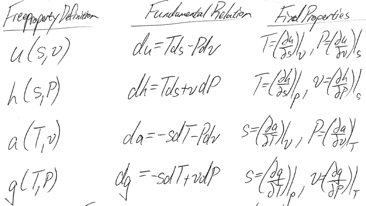
From just one of these four potentials (u,h,a,g) and just two of our four state properties (T,P,v,s) we can estimate all other thermodynamic properties via fast differentials. This is the reason we use Helmholtz explicit EOS instead of Pressure explicit EOS.
We review the methods applied for developing modern, reference quality EOS. We apply the fundamental property rules by programming a real-fluid Helmholtz EOS and calculating properties of interest via common derivatives. Thermodynamic property trees can be developed to show the emergence of new properties that can be useful in determining proper EOS behavior. We also see how, via tools like the general theory of corresponding states, we can fit similar EOS for entire classes of fluids via reducing parameters and rules.
Finally we arrive at mixtures. The primary difference in mixtures is the need to account for varying molar composition of the constituents. We follow the arc of increasing complexity through the following layers:
- ideal-gas mixtures: where the constituents have no idea they are mixed.
- moist-gas mixtures: i.e. psychrometrics, where one component of the ideal mixture becomes condensible. We then realize that this technique is applicable to much more than air-water vapor mixtures.
- real-fluid ideal-solution mixtures: where the individual constituents in the mixture are far from ideal (Z<<1) but are an ideal solution such that no mixture-induced non-idealities occur. In this instance simple mixing rules like Kay’s Law and Amagat’s Law can estimate mixture properties.
- real-fluid non-ideal mixtures: we use the thesis of Konynenburg and the generalized van der Waals EOS to show how many classifications of mixtures emerge from considering the differences in molecule size, critical point, and enthalpy of mixing. These result in the appearance of azeotropes. But with some simple calculations we can estimate a class and difficulty for the mixture we are presented.
- reference quality mixture EOS: we extend the techniques used for developing reference quality Helmholtz EOS into real-fluid non-ideal mixtures like natural gas. The gold standard for accuracy, but you are likely reliant on software for implementation.
The end result is an understanding for the origins of thermophysical property information and understanding the optimal sources of information based on the needs of a particular problem.
Transport, Non-Equilibrium Thermodynamics, and Entropy/Energy Optimization
In this final third of class we show the origins of transport rooted in the second law of thermodynamics and the thermodynamic property of residual entropy. Residual entropy, or the non-ideal contribution to the total entropy in fluid systems that results from particle interactions, is a key predictor of transport properties such as kinematic viscosity and thermal conductivity.
In our early review of introductory thermodynamics we were unsettled in the origins of entropy generated by heat transfer through a finite temperature gradient. Why was the entropy flow into or out of the system a function of the system boundary? We can now revisit entropy generation due to fluxes and driving forces, Onsager’s original insight that created the field of non-equilibrium thermodynamics:
Sgen = ∑(dS/dvar)(dvar/dt) > 0
Where dS/dvar is the driving force, or change in entropy with an independent variable (var), and the flux or change in that independent variable with time (t). Entropy generation from fluxes and driving forces leads to the mathematical structure of all transport phenomena — a flux is defined by the product of the conductance and the spatial gradient:
- Thermal Diffusion: q”=-k(∂T/∂x) where q” is the heat flux, k the thermal conductance, ∂T/∂x the spatial temperature gradient.
- Chemical Diffusion: j”=-D(∂c/∂x) where j” is the mass flux, D is the diffusion coefficient, ∂c/∂x is the spatial concentration gradient.
- Electrical Diffusion: i”=-ec(∂V/∂x) where i” is the electrical current flux, ec is the electrical conductivity, and ∂V/∂x is the spatial electrical potential (voltage).
- Mass Diffusion: m”=-lp(∂P/∂x) where m” is the mass flux, lp is the flow coefficient, and ∂P/∂x is the spatial pressure gradient driving the flow.
- Momentum Diffusion: tau”=-eta(∂vx/∂y) where tau” is the xy-element of the viscous pressure tensor tau, eta is the shear viscosity and ∂vx/∂y is the spatial velocity gradient.
Onsager’s original breakthrough was the realization that when close to equilibrium, reciprocity of these diffusion mechanisms results from coupling to the second law of thermodynamics: Lij=Lji. This means that the entropy optimization of any system results in the consideration of competing and coupled entropy generation mechanisms.
Relevant Blogs
-
ME 527 Lesson 25: Corresponding States
We’re now shifting gears, and deviating from the syllabus, to touch on a classic topic that will set the stage for our Fluid Friday discussions this Friday.
A fantastic book … » More …
Read Story -
The not so ideal later days of thermophysical properties
Last time we discussed the ideal early days of thermophysical properties. Specifically we looked into the progression of the ideal gas law by the natural philosophers and eventually physicists … » More …
Read Story -
The ideal early days of thermophysical properties
Flash back to the literal days of Sir Isaac Newton and horse drawn carriages. Natural Philosophy was the hobby of the wealthy elite. It is in these humble beginnings that … » More …
Read Story